Implementation and Experiments

Two different architectures

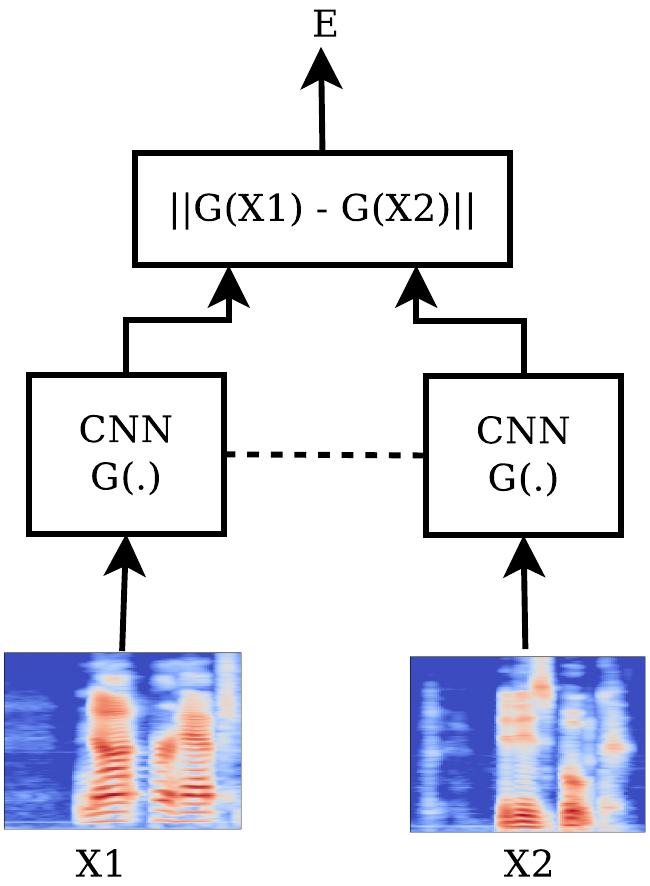
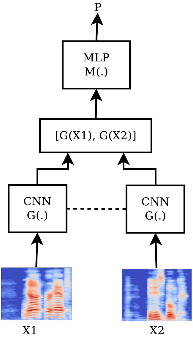
Two different architectures, depicted in the following figures - let’s call them SC-CON and SC-ENT - were tried.

___________

SC-CON (left) and SC-ENT (right) architectures for the implementation of the Siamese Network.

At each case, the architecture of the tied subnetworks used was the same and consisted of $3$ convolutional blocks ($32$, $64$, and $96$ filters) followed by $3$ dense blocks ($384$, $192$, and $96$ neurons). Each block had a batch normalization layer, as well as a dropout layer with $p=0.1$. The activation function used was ReLU, while the kernels were initialized based on Xavier initialization. For all the convolutional blocks, the size of the convolution window was $3\times3$ and the stride was equal to $1$ at both dimensions, while a max pooling of size $2\times2$ was applied. The corresponding Python function (using the Keras API) is:

from keras.models import Model
from keras.layers import Input, Conv2D, BatchNormalization, 
                         Activation, MaxPooling2D, Dropout, 
                         Flatten, Dense

def create_subnetwork(input_shape):
  # Subnetwork to be shared by the siamese architecture.
  
  input_layer = Input(shape=input_shape)

  x = Conv2D(32, (3,3), strides=(1,1), padding='same', 
             kernel_initializer='glorot_normal', 
             kernel_regularizer=None)(input_layer)
  x = BatchNormalization()(x)
  x = Activation('relu')(x)
  x = MaxPooling2D(pool_size=(2,2))(x)
  x = Dropout(0.1)(x)

  x = Conv2D(64, (3,3), strides=(1,1), padding='same', 
             kernel_initializer='glorot_normal', 
             kernel_regularizer=None)(x)
  x = BatchNormalization()(x)
  x = Activation('relu')(x)
  x = MaxPooling2D(pool_size=(2,2))(x)
  x = Dropout(0.1)(x)

  x = Conv2D(96, (3,3), strides=(1,1), padding='same', 
             kernel_initializer='glorot_normal', 
             kernel_regularizer=None)(x)
  x = BatchNormalization()(x)
  x = Activation('relu')(x)
  x = MaxPooling2D(pool_size=(2,2))(x)
  x = Dropout(0.1)(x)

  x = Flatten()(x)
  x = Dense(384, kernel_initializer='glorot_normal')(x)
  x = BatchNormalization()(x)
  x = Activation('relu')(x)
  x = Dropout(0.1)(x)

  x = Dense(192, kernel_initializer='glorot_normal')(x)
  x = BatchNormalization()(x)
  x = Activation('relu')(x)
  x = Dropout(0.1)(x)

  x = Dense(96, kernel_initializer='glorot_normal')(x)
  x = BatchNormalization()(x)
  x = Activation('relu')(x)
  x = Dropout(0.1)(x)

  return Model(input_layer, x)

where for our purposes input_shape = (128, 128, 1).

For the SC-CON architecture the euclidean distance between the two $96$-dimensional outputs was being computed and the network was trained based on the minimization of the contrastive loss function. Thus, the output of the system was a distance between the inputs (very dissimilar inputs were expected to yield big distances). The contrastive loss is defined as

$L = (1-Y)E^2 + Y\max\{0, m-E\}^2$

where

$E = ||G(X_1) - G(X_2)||$

with $X_1$, $X_2$ the two inputs and $Y$ beign equal to $0$ if the two inputs are labeled “similar” and $1$ otherwise. The margin $m$ is a design parameter which was chosen $m=1$.

For the SC-ENT architecture the two $96$-dimensional outputs were being conctenated into a $192$-dimensional layer which was being propagated successively to a $96$-dimensional dense layer, a batch normalization layer, a ReLU activation layer, a dropout layer with $p=0.1$, and a final $1$-dimensional dense layer. A sigmoid activation function was being applied to that final neuron and the network was trained based on the minimization of the binary cross-entropy loss function. Thus, the output of the system was essentially the likelihood that the two inputs are similar or not.

The model described for those two cases can be generated by the following function:

from keras.layers import Lambda, Concatenate
from keras import backend as K

def euclidean_distance(vectors):
  x, y = vectors
  return K.sqrt(K.maximum(K.sum(K.square(x - y), axis=1, keepdims=True), K.epsilon()))

def create_siamese_network(input_shape, architecture):
  subnetwork = create_subnetwork(input_shape)

  input_layer1 = Input(shape=input_shape)
  input_layer2 = Input(shape=input_shape)

  # use the same instance of subnetwork (with different inputs)
  # so, in effect use the same subnetwork (same weights) => siamese
  suboutput1 = subnetwork(input_layer1)
  suboutput2 = subnetwork(input_layer2)

  if (architecture == 'sc-con'):
    # works with Tensorflow backend
    out_distance = Lambda(euclidean_distance)([suboutput1, suboutput2])
    model = Model([input_layer1, input_layer2], out_distance)

  elif (architecture == 'sc-ent'):
    merged = Concatenate(axis=-1)([suboutput1, suboutput2])
    x = Dense(96, kernel_initializer='glorot_normal')(merged)
    x = BatchNormalization()(x)
    x = Activation('relu')(x)
    x = Dropout(0.1)(x)
    x = Dense(1, kernel_initializer='glorot_normal')(x)
    likelihood = Activation('sigmoid')(x)
    model = Model([input_layer1, input_layer2], likelihood)

  return model

Two different testing approaches

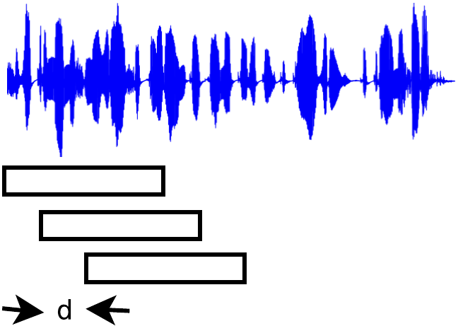
Any recording where it was desired that the speaker homogeneous regions be found by the trained system had to be split into consecutive segments of the same duration as the training segments ($1.27$sec) and each segment had to be preprocessed with the same feature extraction technique applied during the training. Adjacent segments could then be compared throught the network to decide whether the segments belong to the same or different speakers. “Adjacent” segments can be defined in two different ways as shown in the following figures.

____

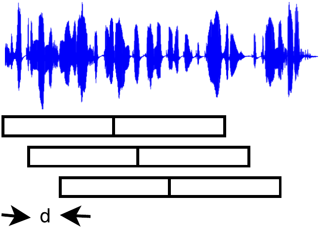
Two different point of views about adjacent segments. (left): The signal is windowed in overlapping segments and 2 consecutive segments form a pair. (right): The signal is windowed in overlapping segments but each pair is formed by non-overlapping segments.

Evaluation Metrics

The evaluation metrics traditionally used for SCD are the False-Alarm Rate ($FAR$) and the Mis-Detection Rate ($MDR$), as well as the $precision$, $recall$, and $F_1$-score, as defined by the following formulas:

$FAR = \frac{\text{#false_alarms}}{\text{#false_alarms + #correct_detections + #missed_detections}}$ $MDR = \frac{\text{#missed_detections}}{\text{#correct_detections + #missed_detections}}$ $precision = \frac{\text{#correct_detections}}{\text{#correct_detections + #false_alarms}}$ $recall = \frac{\text{#correct_detections}}{\text{#correct_detections + #missed_detections}}$ $F_1 = 2\frac{precision \cdot recall}{precision + recall}$

A tolerance margin is also traditionally applied, since it is nearly impossible to find the “perfect” timestamps of a speaker change, as labeled by human annotators. This tolerance margin has been seleceted equal to $\pm0.5$sec, which is a typical value.

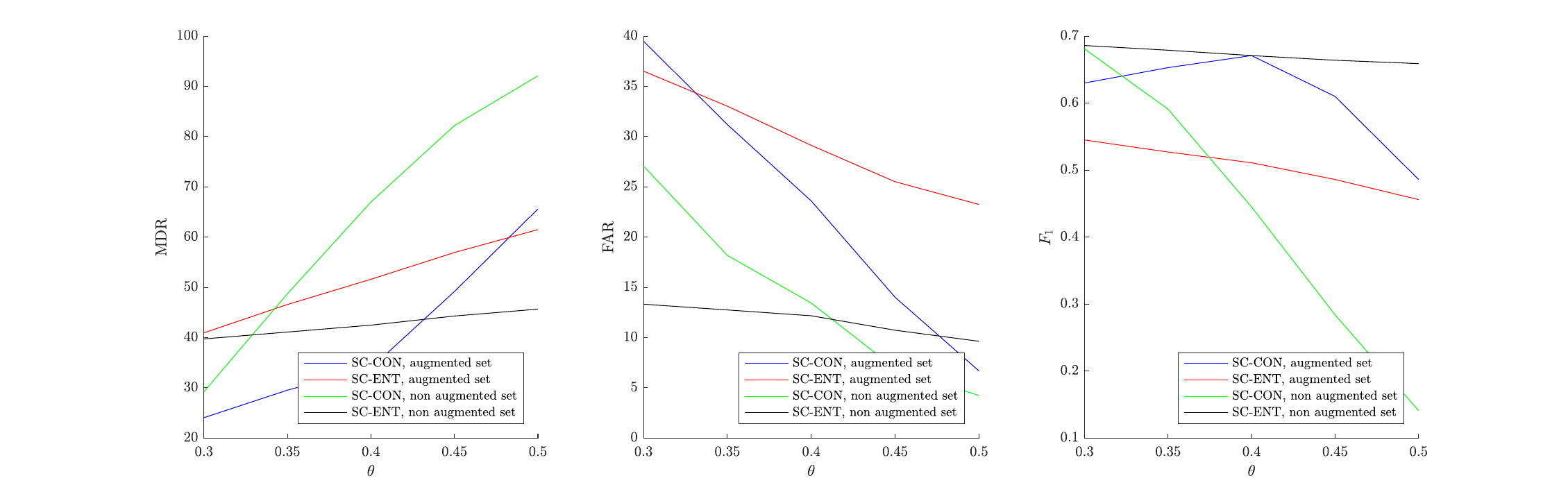
Results

First of all let’s take a look at some training curves to get some insight about the speed and the convergence of the network under the different approaches (SC-CON and SC-ENT, using the augmented training dataset or only the original one). Here, accuracy is referred to the binary problem of whether the input pairs of segments belong to the same speaker or not.

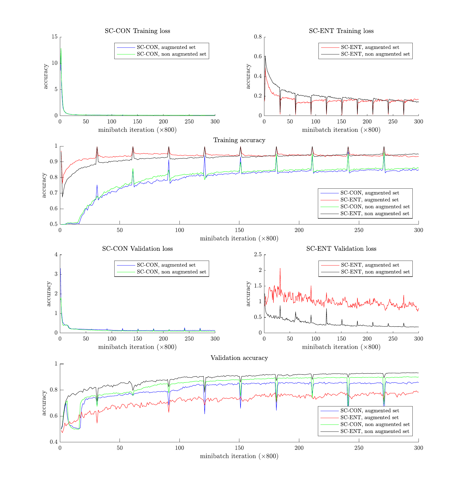
It is observed that in the case of the SC-ENT architecture the convergence (in terms of the training loss minimization) is significantly faster when using the augmented data. However, the final performance is consistently better without any augmentation. Additionally, it seems that SC-ENT yields better results than SC-CON.

For the testing set, it was observed during initial experimentation that the second approach described (comparing non-overlapping consecutive segments) was giving significantly better results, so those are the only ones which are going to be presented here. Specifically, the testing recording was split into small chunks as explained previously with a time shift of $d=0.1$sec. Adjacent segments were being compared and when the likelihood (for SC-ENT) or the distance (for SC-CON) was bigger than a specified threshold $\theta$ it was decided that the segments belong to different speakers. A smoothening postprocessing was applied by not allowing two consecutive speaker changes happening in less than 0.2sec. If consecutive speaker turns were found with distance less $0.2$sec between them, only one speaker turn was kept and it was assumed that it happened in the time average of all those speaker changes that the algorithm found.

In order to find an “optimal” threshold $\theta$ the initial idea was to randomly create multiple validation sets, find the best threshold on them based on a grid search and take the average value. However, it was observed that this threshold was highly dependent on the testing dataset. Thus, the results are presented here for multiple values of the threshold $\theta$.

SC-SCD

Siamese Convolutional Networks for Speaker Change Detection

Implementation and Experiments

Two different architectures

Two different testing approaches

Evaluation Metrics

Results